Parameter Sweeps with EnsembleProblem

One of the most powerful features of the PottsToolkit design is that PottsProblem is a first-class citizen of the SciML ecosystem. This means that SciMLBase.EnsembleProblem works out of the box — no adapter code, no monkey-patching. In this tutorial we sweep the Metropolis temperature T over four values, solve the same cell-sorting model for each, collect a cluster-size metric, and plot how temperature controls the degree of cell sorting.

Packages

using PottsToolkit
using SciMLBase
using Statistics
using CairoMakie
CairoMakie.activate!()   # or GLMakie / WGLMakie

Base model

We define a two-population sorting system (A and B cells prefer their own kind) and a base PottsProblem. Each ensemble member will modify only the algorithm temperature while sharing the same system.

A = CellType(:A)
B = CellType(:B)
Medium = CellType(:Medium, is_background = true)

sys = PottsSystem(
    cell_types = [Medium, A, B],
    penalties = [
        VolumeComponent(
            A => (λ = 5.0f0, target = 500),
            B => (λ = 5.0f0, target = 500)
        ),
        AdhesionComponent(
            (A, Medium) => 16.0f0,
            (B, Medium) => 16.0f0,
            (A, A) => 2.0f0,
            (B, B) => 2.0f0,
            (A, B) => 14.0f0
        )
    ]
)

base_prob = PottsProblem(
    sys,
    Dict(A => 25, B => 25),
    (200, 200);
    tspan = (0, 600),
    topology = VonNeumannTopology{2}()
)

Temperature sweep values

temperatures = [0.5f0, 1.0f0, 2.0f0, 4.0f0]

4-element Vector{Float32}:
 0.5
 1.0
 2.0
 4.0

Ensemble setup

prob_func receives the base problem and the ensemble index i; it returns a modified problem or a new algorithm. Here we bundle algorithm + problem into a named tuple via the SciMLBase.EnsembleProblem prob_func / output_func interface. The standard pattern stores the temperature in the metadata and reconstructs the algorithm inside prob_func.

function output_func(sol, i)
    # Compute a scalar sorting metric: mean size of contiguous same-type clusters.
    # type ID 1 = A (first non-background type, in declaration order)
    final_state = sol.u[end]
    n = final_state.N_cells[]
    types = Array(final_state.cell_data.cell_types)
    a_cell_ids = Set(findall(==(1), types[1:n]))
    grid = Array(final_state.grid)
    Nx, Ny = size(grid)
    tile = 20
    densities = Float64[]
    for ix in 1:tile:(Nx - tile), iy in 1:tile:(Ny - tile)

        block = grid[ix:(ix + tile - 1), iy:(iy + tile - 1)]
        push!(densities, mean(x -> x ∈ a_cell_ids, block))
    end
    metric = std(densities)   ## higher std → more sorted
    return (metric, false)
end

ensemble_prob = SciMLBase.EnsembleProblem(
    base_prob;

    output_func = output_func
)

Run the sweep

We use EnsembleSerial for reproducibility. Switch to EnsembleThreads for a free speedup on multi-core machines.

results = Vector{Float64}(undef, length(temperatures))

for (i, T) in enumerate(temperatures)
    alg = CheckerboardMetropolis(T = T, sweeps_per_step = 10)
    sim = SciMLBase.solve(
        ensemble_prob, alg, SciMLBase.EnsembleSerial();
        trajectories = 1,
        saveat = 60
    )
    results[i] = sim.u[1]   ## output_func returned the scalar metric
end

Plot results

Higher temperature → less sorting → lower spatial variance of cell-type density.

fig = Figure(resolution = (700, 450))
ax = Axis(fig[1, 1];
    xlabel = "Metropolis Temperature T",
    ylabel = "Sorting index (std of A-density per tile)",
    title = "Cell Sorting vs. Temperature"
)
scatterlines!(ax, Float32.(temperatures), results;
    color = :steelblue,
    markersize = 12,
    linewidth = 2
)
save("parameter_sweep_sorting.png", fig)
fig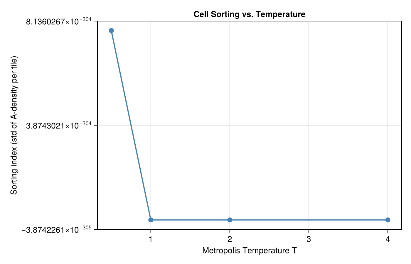

This page was generated using Literate.jl.